Audio Visualizer

Overview

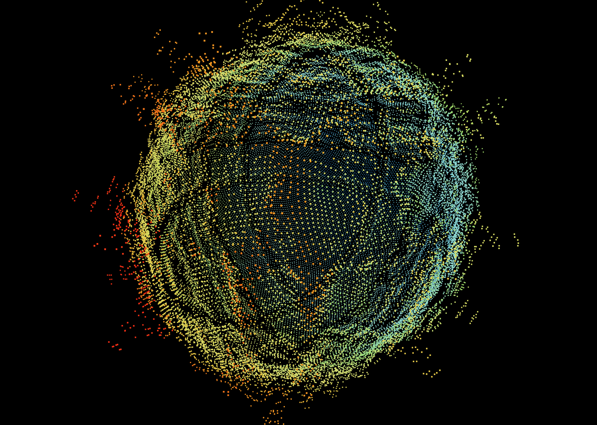
This Audio Visualizer is a browser-native implementation of a custom real-time three-dimensional audio visualization algorithm. Live audio is captured and processed for analysis via the Web Audio API, and fed as input into the visualization algorithm. Any audio source can be used, and will drive the real-time deformation of a point cloud.

Setting aside the techniques used to extract and stage the audio for consumption, there are several defining components to the actual visualization process, which are agnostic to the web-based implementation:

1. Initial creation and formation of the point cloud
2. Point cloud pre-processing and frequency responsibility mapping
3. Continuous audio-driven real-time deformation of the point cloud

Point Cloud Generation

The initial creation and formation of the point cloud is the first step in the visualization process. In this instance, a sphere is dynamically generated using a Fibonacci spiral algorithm based on a specified number of points, which evenly distributes points across the surface of a sphere avoiding polar clustering and gaps in coverage. The more evenly distributed the points are, the more visually appealing and stable the resulting point cloud will be.

The visualization process is actually entirely agnostic to the underlying shape of the point cloud; I used a sphere for two main reasons:

1. The simpler the shape, the more readable and clear the point deformations will be. Given a sufficiently complicated shape, the deformations become less perceptible and visually muddy. A sphere is a simple shape where all points will have a unique normal axis of deformation, making deformation paths non-intersecting and distinct.
2. It was easy to generate a sphere, and allowed me to focus most of my time on the more salient portions of the visualization process.

It is technically trivial to accept a different set of points either through additional generation algorithms or by accepting an uploaded point cloud file. I may eventually add this feature to the web-based implementation, but for now I have been having more fun focusing on refining the pre-processing and deformation algorithms.

Point Cloud Pre-Processing and Frequency Responsibility Mapping

Two main types of deformation occur for every point: positional, and color-based. If every point deformed identically, the visualization would lack depth and appeal. In order to diversify how each point deforms, a pre-processing step iterates over every point and calculates a set of parameters that will be used during the actual deformation phase. Pre-processing these parameters is critical to ensuring the algorithm can run in real-time with as little latency as possible, since there are often thousands of points in the point cloud to process as fast as possible per-frame.

The first and most important parameter for each point is the frequency responsibility mapping. As a component of the deformation algorithm, each point will incorporate the amplitude of certain frequencies it was assigned during this pre-processing stage. During pre-processing, each point on the sphere uses its initial coordinates to determine the specific frequencies it should react to in the audio data. The result of this step of the pre processing is a set of indexes into the FFT data array that the point will reference per-frame during execution of the deformation algorithm. Currently, simple axis-based mapping is used, but I eventually plan to incorporate different mapping techniques like Poisson disk sampling, spherical harmonics, and more.

The second parameter that is pre-processed is the initial color gradient. At rest, every point on the sphere has an original static color. During deformation, the color will change, but the origin color itself determines the range of the color change function. During the pre-processing phase, each point is assigned a color based on its position on the sphere, resulting in a gradient of colors that serve as the foundation for the color deformations. Since the resting color for each point is originally different across the sphere, the color variety will remain diverse and interesting.

The original positions and colors of all points are stored in memory at the end of pre-processing. This allows the animation logic to apply deformations relative to the initial state, ensuring that all transformations are reversible and that the visualization can respond smoothly to changes in audio (and user settings, for the web-based implementation).

Point Deformation Algorithm

At each animation frame, every point's position and color are updated based on a combination of four audio-reactive terms. By summing these contributions and multiplying by the unit normal for every point, the entire shape deforms in time with the sound.

1. Noise wave - A low-frequency sine function consistently applies a slow and gentle deformation, providing for interesting movement even when the audio is quiet. The noise parameters can also be adjusted to fundamentally change the underlying shape and make it more dynamic.
   sin(t * noiseWaveSpeed + φ_i * noiseWaveFreq) * noiseWaveAmp

   • t: the clock's time in seconds
   • noiseWaveSpeed: how fast the entire sine wave oscillates over time (controls “breathing” rate).
   • φ_i: the point's latitude angle, computed as acos(1 - 2(i+0.5)/count). This spreads out phase shifts so points across the sphere reflect different parts of the wave.
   • noiseWaveFreq: the frequency of the sine wave. Effectively, how quickly the phase φ_imodulates the sine wave over the surface of the sphere.
   • noiseWaveAmp: the amplitude of the sine wave. Effectively, the maximum radial kick (displacement) any point can get from this single noise term.
2. Bass wave - A second sine wave is applied across the entire shape whose frequency is driven by dampened bass intensity and whose amplitude scales exponentially with raw bass.

   Without the bass wave, the visualization can appear underwhelming when reacting to audio with loud bass frequencies. To a human, heavy bass feels very energetic and powerful. Mathematically, however, bass frequencies take up a very small portion of the audible spectrum. Even if lower frequencies are logarithmically mapped across the shape, only a relatively small portion of the sphere would directly react to high-amplitude bass frequencies. I found that it always lacked a certain "oomph" when only the points responsible for visualizing bass frequencies would move, and other points would seem unaffected, when from an intuitive experience standpoint, I felt the sphere should be more energetic. The bass wave reflects this implicit energy by deforming the entire sphere in response to bass frequencies, outside of the normal frequency mapping pipeline.

   sin(t * bassSpeed + φ_i * (maxFreq * dampenedBassIntensity)) * (maxAmp * rawBassIntensity ** (1/responseCurve))

   • dampenedBassIntensity: value controlling the frequency of the bass wave. It is derived from the raw bass intensity: dampenedBassIntensity = max(0, rawBassIntensity - normalizedAvgVolume * C).

     When the dampened bass intensity value is higher, the frequency of the bass wave approaches its maximum value (making the bass wave effect more pronounced). The bass intensity is dampened before affecting the frequency to prevent the bass wave from overwhelming the visualization when average volume is high. The bass wave is most important when the dominant frequencies are bass frequencies, and not much else is going on in the other frequency bands. If there is already a lot of information to represent in the other frequency bands, the bass wave can overwhelm the surface of the point cloud if its effect is not tempered. By reducing the effect the bass intensity has on the wave by the average volume across all frequencies, the bass wave is only pronounced in situations where there is a lack of energy and "oomph" provided from the other frequencies.

     Because this term affects the frequency of the bass wave, the ripples generated by the bass wave appear to oscillate back and forth laterally across the sphere in correlation with bass frequency amplitudes. This lends another dimension to the visualization that amplitude controls (in addition to the normal radial displacement driven by amplitude).

   • maxFreq: the maximum frequency of the bass wave.
   • rawBassIntensity: average amplitude of the lowest FFT bins (0…bassCutoffIndex), normalized to [0,1].
   • responseCurve: shapes amplitude sensitivity. (> 1: boosts low bass, <1: compresses).
   • maxAmp: peak displacement from bass wave.
   • bassSpeed: time multiplier for bass-wave oscillation. At a fixed dampened bass intensity, the bass wave would traverse across the surface of the sphere at this rate.
3. Global volume push - A uniform radial expansion proportional to overall loudness:
   avgVolume * volumeConstant * volumeScale

   • avgVolume: mean of all FFT bins (0…255).
   • volumeConstant: fixed value, (maps 0-255 into a reasonable values that can be directly used in the spatial rendering system to perform displacement).
   • volumeScale: sensitivity multiplier for global volume push.
4. Frequency-specific displacement - Fine, localized surface displacement driven by a point's frequency responsability mapping:
   calculateFrequencyScale( reduceAmplitude(binX_i), reduceAmplitude(binY_i), reduceAmplitude(binZ_i) ) * freqConstant * frequencyScale

   • binX/binY/binZ: the FFT indices assigned to this point during preprocessing for each axis.
   • reduceAmplitude(): soft-clips low amplitudes below afrequencyMinimum via an exponent. (Frequency damping)
   • calculateFrequencyScale(): based on the number of active frequency mappings (axes) and constituent frequency amplitudes, intelligently combine the amplitudes and output a scale value to use for point displacement. Since frequency mappings can be conditionally enabled/disabled in this implementation, dynamic tuning is required to ensure the scale value generated is reasonable.
   • frequencyScale: sensitivity multiplier for frequency-specific displacement.

These four terms are summed into a single scale value, and applied to the normal axis of that point:

scale = radius (original position) + wave + bassWave + volDisp + freqDisp

newPosition = normalVector.multiplyScalar(scale)

Once positionally displaced, the point is re-colored based on the magnitude of its displacement from its original position. A function is used to smoothly shift the point's hue toward its complementary color in proportion to how far it has moved beyond the rest radius. I am still not quite satisfied with the current behavior, and the exact calculation is still the subject of my tinkering so I won't get into too much detail here (yet...)

After computing each point's new position and color, a slow spin is applied to the entire point cloud. The angular velocity in each axis is multiplied by a momentum value, which is the average volume itself multiplied by a sensitivity constant. Effectively, bursts of volume letting loud moments “kick” the sphere faster. Truthfully its less of a momentum value and more of an instantaneous speed-up effect, but I named it momentum when I first implemented it and the name stuck.

Web Implementation

I implemented the entire algorithm as a web page because I wanted to experiment and play around with the algorithm in real time, and make it easy and accessible for others to do the same. The live demo includes a user-friendly control panel exposed on the UI (built with Leva) that lets visitors tweak a lot of the core parameters of the algorithm in real time. Orbit controls enable interactive camera rotation and zoom, and all settings are hot-reloaded so you can instantly see how each adjustment you make affects the visualization. Not every single parameter of the algorithm is exposed but all of the core functionality is tweakable and available to play around with. I would encourage you to try it out yourself!

I also implemented a spectrogram you can use to inspect the audio signals that your browser is consuming from your selected audio source.

Looking Ahead

There is still a lot to explore in this project. In no particular order, some things I am still working on for this project are:

• Frequency mapping methods (Poisson, spherical harmonics, etc.)
• Improvements and fixes to the color mapping and color transformation algorithm
• Changes to the positional deformation algorithm
• Performance optimizations
• More complex point cloud generation algorithms (e.g. toroidal, fractal, etc.)

Technologies Used

• Core Stack – Next.js 14 (App Router), React 18, TypeScript; built on the T3 Stack with Tailwind CSS (scaffolded project-wide, not directly used in the visualizer). The main visualization logic is implemented in TypeScript, leveraging React hooks for state management and lifecycle handling.
• 3D Graphics – Three.js via react-three-fiber for declarative WebGL scene management and high-performance point-cloud rendering.
• Audio Analysis – Web Audio API’s AnalyserNode for real-time FFT; custom useAudioStream hook handles device selection, stream setup, and frequency data.
• UI & Styling – Tailwind CSS utility classes and custom global styles; Leva for live parameter panels; Radix UI primitives for accessible dialogs/tooltips; Heroicons & react-icons for iconography.
• Utilities & Debugging - Modular math and color utilities implemented in TypeScript for displacement and hue logic; StatsForNerds component for runtime audio/visual stats.
• Build & Documentation – Next.js build system with standard npm scripts; project deployed and hosted on Vercel.

Project Links